This is the second lecture for ENGN 2210: Continuum Mechanics, guest-taught by my labmate Aashutosh. Course materials will be available on the course website.
This lecture introduces the concepts of maps and tensors in a way that is quite different from how I learned them before.
Maps
Definition 3.1: Maps
A map f:X→Y assigns each element of the set X to exactly one element of the set Y. In other words, it returns a single, unique output when operated on an input.
Interestingly, a map f:D⊆R→R is typically referred to as a function, where D is its domain. A function may be specified by a formula, for example,
It is important to distinguish between the function f itself and its function values f(x). The function f is a map, while f(x) denotes the output corresponding to a particular input x. The collection of all possible function values forms the range of the function.
A map is a more general concept than a real-valued function. It describes a correspondence from one set to another and is not restricted to subsets of the real numbers. Many operations we have already encountered, such as inner products and norms, can also be viewed as maps.
Definition 3.2: Map between Euclidean spaces
The map T:En→Fn assigns each vector v∈En to a unique vector T(v)∈Fn. It is therefore a map between two Euclidean spaces. Here, n denotes the dimension of the Euclidean spaces, and the bold symbol T denotes the map itself, analogous to a function acting between two spaces.
Linear Maps
Definition 3.3: Linear map
A linear map T:V→W is a map between two vector spaces that preserves vector addition and scalar multiplication,
T(u+v)=T(u)+T(v),
for all u,v∈V, and
T(au)=aT(u),for all a∈R and u∈V.
Equivalently, a linear map preserves any linear combination:
T(au+bv)=aT(u)+bT(v).Here, V is the domain and W is the codomain. A linear map is also called a linear transformation.
Note that the definitions of vector addition and scalar multiplication in V and W do not have to be identical.
The set of all linear maps from V to W is denoted by L(V,W).
Here are some examples of linear maps. The identity map satisfies Iv=v, while scalar multiplication by a fixed scalar a gives Tv=av. Writing T(v) instead of Tv can make it clearer that T is a map acting on v.
Differentiation is itself a map defined on a function space. For example,
D:C1(R)→C(R),D(f)=f′.Here, f is one possible input of the map D. The differentiation operator D is defined independently of any particular function f. it assigns each differentiable function to its derivative.
Definition 3.4: Addition and scalar multiplication on L(V,W)
The set of linear maps L(V,W) is itself a vector space if addition and scalar multiplication are defined pointwise as
(S+T)(v)=S(v)+T(v),(aT)(v)=aT(v).Therefore, linear maps can themselves be regarded as vectors in the vector space L(V,W). This emphasizes that a vector is, more generally, an element of a vector space rather than merely a quantity with magnitude and direction.
Properties of linear maps
If S∈L(U,V) and T∈L(V,W), their composition is another linear map
TS∈L(U,W),(TS)u=T(Su).Thus, S acts first and T acts second. Linear-map composition satisfies the usual associative, distributive, and identity properties.
A linear map of the form
T:V→Vis called a linear operator, since its domain and codomain are the same vector space. A linear map of the form
T:V→Ris called a linear functional or linear form.
By the way, linear maps are generally not commutative, so in general,
TSu=STu.However, some particular pairs of maps may commute, meaning that
TS=ST.Whether two maps commute depends on the specific maps and the spaces on which they act.
Tensors
For the time being, we will leave aside a more precise and comprehensive discussion of tensors and, for our present purposes, simply regard them as linear maps between Euclidean vector spaces.
Definition 4.1: Tensors
For our present purposes, we refer to linear maps
T∈L(En,Fn)as tensors, where En and Fn are Euclidean vector spaces. Therefore, the properties previously introduced for linear maps also apply to tensors.
In continuum mechanics, important examples include the deformation gradient tensor, velocity gradient tensor, strain tensors, stress tensors, and stiffness tensors. Since tensors are treated as linear maps here, the set of tensors between two fixed Euclidean vector spaces also forms a vector space.
Definition 4.2: Identity tensor
The identity tensor I:En→En maps every vector to itself:
Iv=v,∀v∈En.It is simply the identity map viewed as a tensor.
Definition 4.3: Null tensor
The null tensor 0:En→Fn maps every vector in En to the zero vector in Fn:
0v=0F,∀v∈En.It is simply the zero map viewed as a tensor.
Note that the two symbols 0 here represent different objects. The 0 on the left denotes the null tensor, i.e. the zero element of the tensor space L(En,Fn), while 0F on the right denotes the zero vector in the codomain Fn.
Definition 4.4: Transpose of a tensor
The transpose of a tensor T is the tensor TT defined by
u⋅(Tv)=(TTu)⋅v,∀u,v∈En.In other words, the transpose transfers the action of T from one side of the inner product to the other.
Note that this is the definition of the transpose tensor, not merely a property derived from its matrix representation. This relation is often useful in proofs, since it allows T to be moved from one side of the inner product to the other as TT.
The transpose satisfies several useful algebraic properties:
(AT)T=A,(AB)T=BTAT,(A+B)T=AT+BT,(αA)T=αAT.In particular, note that the transpose reverses the order of a product.
Definition 4.5: Symmetric tensors
A tensor T is symmetric if \bm T = \bm T^\rm{T}:KaTeX parse error: Got function '\rm' with no arguments as superscript at position 15: \bm T = \bm T^\̲r̲m̲{T}.
Definition 4.6: Skew-symmetric tensors
A tensor T is skew-symmetric if
T=−TT.Every tensor can be uniquely decomposed into the sum of a symmetric part and a skew-symmetric part:
T=sym(T)+skew(T),where
sym(T)=21(T+TT),skew(T)=21(T−TT).Dyadic product
Definition 4.7: Dyadic product
The dyadic product (or tensor product) of two vectors a and b is the tensor a⊗b defined through its action on an arbitrary vector c,
(a⊗b)c=(b⋅c)a.Thus, a⊗b is a linear map that projects c onto b through the inner product b⋅c, and then scales a by that scalar. A tensor of the form a⊗b is also called a dyad.
Note that this is the definition of the dyadic product, and it is often used directly to prove its algebraic properties.
Properties of dyads
The dyadic product satisfies several useful identities:
(a⊗b)T=b⊗a,(a⊗b)(c⊗d)=(b⋅c)a⊗d,(a⊗b)A=a⊗(ATb),A(a⊗b)=(Aa)⊗b.The last two identities can be proved directly from the definition of the dyadic product by applying both sides to an arbitrary vector c.
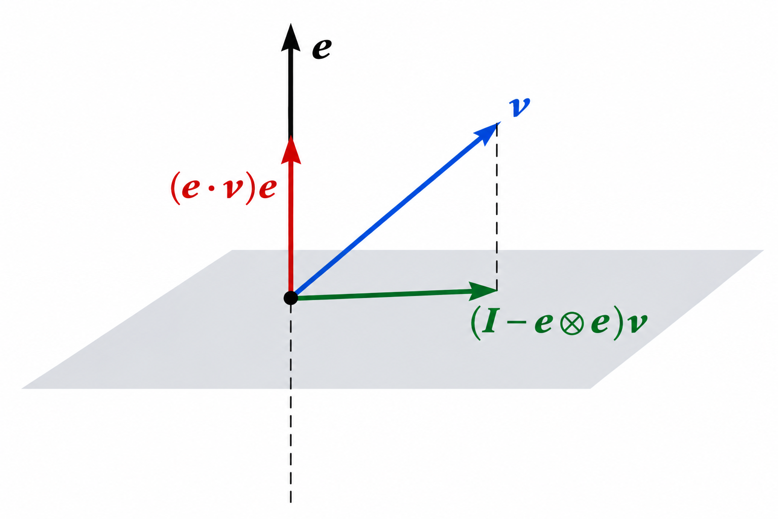
Let e be a unit vector. Then
(e⊗e)v=(e⋅v)eis the projection of v onto the direction of e. Correspondingly,
(I−e⊗e)v=v−(e⋅v)eprojects v onto the subspace parallel to e.
First edited on Sep. 15, 2026. I find it very impressive that tensors are introduced from the perspective of linear maps. I hope this perspective will help me gain deeper insights as I revisit continuum mechanics.