MFEM 01
My first step toward learning MFEM
Overview
Over the past two weeks, I was asked to use MFEM for finite element simulations in fracture mechanics. I did perform a considerable amount of finite element simulation during my master's studies. However, the basic finite element framework in the solver developed by my former group had already been established by my former advisor, Prof. Ju Liu. My own work mainly focused on implementing constitutive models for visco-hyperelasticity.
Recently, I have been exploring MFEM and trying to reproduce the same capabilities that I was familiar with in my former group's code. This has turned out to be much more challenging than I initially expected, with many issues arising along the way. Therefore, I decided to approach MFEM as a complete beginner and start again from some simple problems.
The source code is available on GitHub, and you can also visit the official MFEM website for documentation and additional resources.
In this post, I solve a one-dimensional elastic bar problem and walk through the code in the order in which it is executed, placing each part alongside the corresponding formula it implements. The full code is available at Chongran-Zhao/mfem-solids.
Problem setting
A slender bar of length
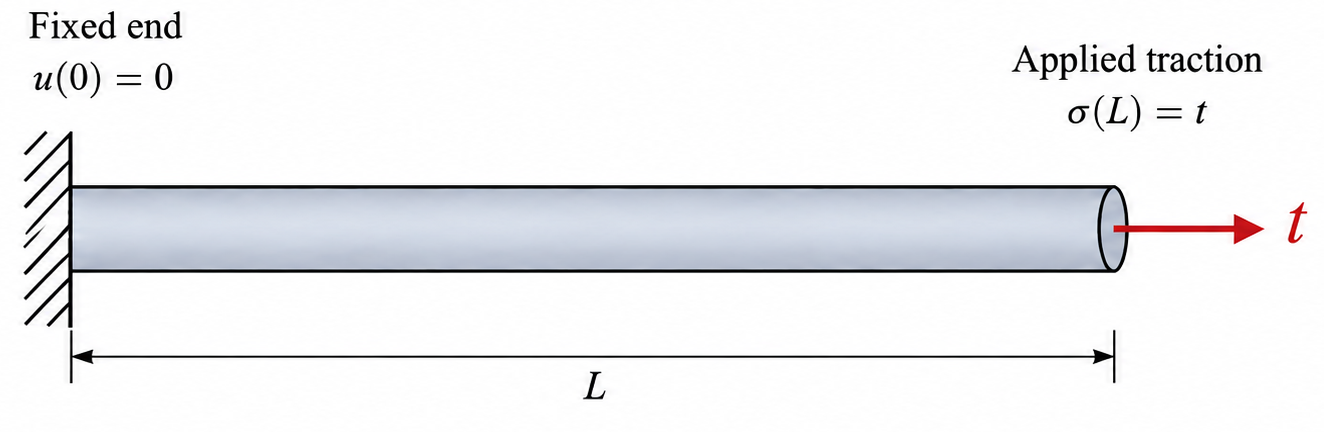
With
1. Problem data
const mfem::real_t length = 1.0;        // L [m]
const mfem::real_t young = 200.0e9;     // E [Pa]
const mfem::real_t traction = 100.0e6;  // t [Pa]
const int num_elements = 4;
const int order = 1;
| Symbol | Variable | Value |
|---|---|---|
length |
1 m | |
young |
200 GPa | |
traction |
100 MPa | |
num_elements |
4 | |
order |
1 |
2. Mesh
mfem::Mesh mesh = mfem::Mesh::MakeCartesian1D(num_elements, length);
- No mesh file is read: the mesh is built in memory.
numbers nodes and numbers elements. Element connects nodes and , which is why a node subscript appears in ; this holds only for such a sequentially numbered 1D mesh. - Boundary attributes are integer labels that the mesh attaches to its boundary elements, so that each piece of the boundary can be referred to by a number.
MakeCartesian1Dlabels the two end points:
| Boundary element | Location | Attribute |
|---|---|---|
| point | 1, i.e. |
|
| point | 2, i.e. |
Every boundary condition below picks its boundary by attribute, not by coordinate: attribute 1 for the fixed end (step 4) and attribute 2 for the traction (step 6). For a mesh read from a file, the file assigns these numbers, and mesh.bdr_attributes lists the ones present, here
3. Shape functions and finite element space
mfem::H1_FECollection fec(order, mesh.Dimension());
mfem::FiniteElementSpace fespace(&mesh, &fec);
fec is the reference element, and it computes nothing. From order and the mesh dimension it only selects which H1_1D_P1 here — and stores its basis on the reference element order = 1 in 1D this is the two-node linear element:
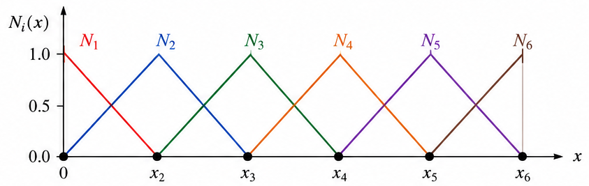
Each element
Both are first order here. The geometry of this mesh is always this linear map, so with order = 2 the field would be quadratic while the geometry stayed linear (subparametric).
fespace is the discrete space, and it is where the mesh enters. It carries the reference basis onto every element through
- It also records which global number each element's local function carries, the table
used in step 5. - A space is not a field:
fespacestores no values. The trial displacement, the test function and any other field of the problem expand in these same , each with its own coefficients. That is why displacement appears only in step 7. vdim, the third constructor argument, is the number of components per basis function: 1 here, andvdim = dimfor 2D or 3D elasticity, which givesvdimunknowns on the same mesh and the same fec.carries no boundary condition yet; that is step 4.
4. Essential boundary condition
mfem::Array<int> fixed_bdr(mesh.bdr_attributes.Max());
fixed_bdr = 0;
fixed_bdr[0] = 1;                       // attribute 1, the end at x = 0
mfem::Array<int> ess_tdof_list;
fespace.GetEssentialTrueDofs(fixed_bdr, ess_tdof_list);
fixed_bdrhas one entry per boundary attribute; its sizebdr_attributes.Max()is 2.- This step only collects indices. Nothing is imposed until step 8.
5. Weak form and stiffness matrix
mfem::BilinearForm stiffness(&fespace);
stiffness.AddDomainIntegrator(new mfem::DiffusionIntegrator);
stiffness.Assemble();
Multiply
Look for
Substitute both into Eq. (4), and use
Both sides are linear in the
Every free
What Assemble() computes on each element: the integral is pulled back to
and how it adds them up, where
BilinearFormis the left-hand side of Eq. (4);DiffusionIntegratoris the integrand, with coefficient 1. Assemble()is the sum over elements: compute, then add it at the global positions , . - The test function is never stored: row
is the equation for .
6. Natural boundary condition and load vector
mfem::ConstantCoefficient scaled_traction(traction/young);
mfem::Array<int> end_bdr(mesh.bdr_attributes.Max());
end_bdr = 0;
end_bdr[1] = 1;                         // attribute 2, the end at x = L

mfem::LinearForm load(&fespace);
load.AddBoundaryIntegrator(new mfem::BoundaryLFIntegrator(scaled_traction),
                           end_bdr);
load.Assemble();
end_bdrmarks where to integrate; in 1D,is a single point. - The essential condition selects unknowns (step 4); the natural condition adds to the right-hand side (step 6).
7. Displacement field
mfem::GridFunction disp(&fespace);
disp = 0.0;
- A
GridFunctionis a function, not just a vector. - The initial value 0 supplies the prescribed
.
8. The linear system
mfem::SparseMatrix stiff_mat;
mfem::Vector solution, rhs;
stiffness.FormLinearSystem(ess_tdof_list, disp, load,
                           stiff_mat, solution, rhs);
Write Eq. (5) in matrix form, splitting the unknowns into constrained
MFEM keeps the full size instead of deleting row and column
For this problem,
disp and load are built on the finite element space: besides their numbers they know the basis solution and rhs are plain vectors, the numbers alone, which is all a solver needs.
built on fespace |
plain vector | what the numbers are |
|---|---|---|
stiffness |
stiff_mat |
|
disp |
solution |
|
load |
rhs |
- Each pair shares memory, so the call rewrites
stiffness,dispandloadin place, and whatever the solver writes intosolutionis already indisp. Here the right column is pure convenience. - The two columns are genuinely different objects only when the solved system is smaller than the space: non-conforming meshes, static condensation, parallel runs.
9. Solving and recovering
mfem::GSSmoother precond(stiff_mat);
mfem::CGSolver solver;
solver.SetRelTol(1e-12);
solver.SetMaxIter(100);
solver.SetPrintLevel(0);
solver.SetPreconditioner(precond);
solver.SetOperator(stiff_mat);
solver.Mult(rhs, solution);

stiffness.RecoverFEMSolution(solution, load, disp);
stiff_mat is symmetric positive definite, so conjugate gradients applies. The Set... calls say what they do; they are needed only because MFEM's defaults, max_iter = 10 and rel_tol = abs_tol = 0, can never be satisfied. SetMaxIter(100) is a safety net rather than a budget: with 4 free unknowns, CG reaches the exact answer in at most 4 iterations in exact arithmetic.
precond is an approximate inverse. It is an operator of its own: in goes a residual GSSmoother produces that
Mult does not multiply. Every MFEM Operator exposes Mult(x, y), meaning "apply me to x, write the result into y", and a Solver is an Operator whose action is applying the inverse. So solver.Mult(rhs, solution) takes the right-hand side in and writes
- The residual is measured in the preconditioner's norm.
abs_tolstays 0 here, so only the relative test matters; it exists for a right-hand side that is already almost zero, where no relative drop is achievable. RecoverFEMSolution(solution, load, disp): the solved vector goes in, the finite element function comes out. Heresolutionanddispshare memory, so nothing is copied; with static condensation or a non-conforming mesh, this is the step that reconstructs the entries the solved system did not carry.
10. Result
for (int ii = 0; ii < mesh.GetNV(); ++ii)
   mfem::out << "x = " << mesh.GetVertex(ii)[0]
             << "   u = " << disp(ii) << '\n';
- The exact solution is linear, so it lies in the finite element space: linear elements reproduce it exactly, at the nodes and everywhere in between.
- With linear elements, node
iiis degree of freedomii, so the loop prints.
First edited on Sep. 15, 2026, at River House.
I find it very helpful to begin with such a simple case. At this stage, however, it is also necessary for me to revisit the fundamentals of finite element theory. Therefore, becoming familiar with the theory and the code simultaneously is especially important to me. My next goal is to extend the present elastostatic problem to elastodynamics.
This blog post was written with the aid of AI agents. I discussed many details with it and tried to make sure that the article still reflects my own reasoning, questions, and thoughts throughout the learning process.